Monday, 6 May 2019

Kaggle Titanic and OAC

Data Science: How do I get started?
In this blog we’re going to show you how to do one of the Kaggle Introduction competitions without needing to learn a new language. 

Who’s Survived?

The competition we’re going to solve is the Titanic, in this we have 2 data sets, train and test. The train dataset has a labelled column, Survived, where 1 = Yes, survived and 0 = No, didn’t survive. To solve this, we’re going to use a Binary Classifier (Supervised Learning Model).

Step 1 – Acquire the Data: Navigate to Kaggle and download the data files from the Titanic Competition. 

 Step 2 – Loading the Data:Drag and Drop the files in Oracle Analytics Cloud to upload them as data sources. 


Step 3 – Enrich the Data: Once the data is loaded, open the data source and look to enrich the data. There are many areas to enrich, Passenger Title, Cabin Level and. Once enriched makes sure you click on “Apply Script”.
Open the Train Data Set: 
Creating the Feature “Title”
Right click on the name column and left click on Split. 
For the first split, use the “,” and increase the “Number of Parts” to 2.
On the new columns “Name Split 2”, Right click and select split again. This time split on “.”. This will create a new column with the Titles in. 

Family Size: 
Right click on “Parch” and select Duplicate. Right click on the new column created and left click on Edit. 
In the edit box, add together Parch, SibSp and 1 in the formula: #Parch + #SibSp + 1. Rename the column to Family Size.

Cabin Level: 
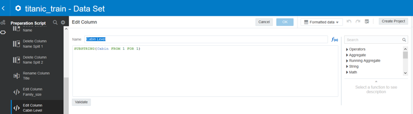
Right click on the column Cabin and left click on “Duplicate”. Right click on the new column created and left click on “Edit”. In the edit screen used the function SUBSTRING to extract the first letter from the cabin data. 

Note: SUBSTRING(<<Column>>, Starting Position, Number of characters to extract)
Step 4 – Augmented Analytics: Left click on “create project”, this will open a blank canvas. One the left-hand side are the data fields. Right click on “Survived” and select “Explain Survived”. 
The explain box will appear on screen and provide a high-level overview of the attribute “Survived”. Left click on the tick in the top right corner. This will indicate the graphs that you want to add to the Canvas. 
Left click on “Key Drivers of Survived”. This will present a number of key drivers towards to the variable “Survived”. Once you’ve selected your graphs, click on “Add Selected”.
This will use Oracle in-built machine learning algorithms to describe the attribute “Survived” and provided detailed visualisations that help to explain the attribute “Survived”.  

Step 5 – Training the model: Once we have explored the data we’re ready to build a machine learning model. On the home screen left click on “Create” and then “Data Flow”. 
The data flow is as follows:
1.    The training data source
2.    Remove any columns not required in the model
3.    Train the Binary Classifier
4.    Save the model 
In this example we’ve built a Neural Network Supervised Learning Model Ensure you select the correct column that you want to predict (“Survived”) and “0” for the positive class in Target (Most Frequent).


Step 6 – Apply the model: From the home screen create a new Data Flow. This data flow will apply the machine learning model you’ve just created to the test data set. 
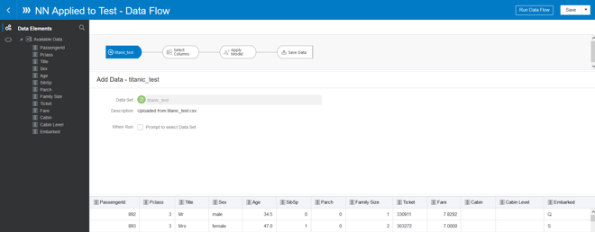
The data flow is as follows:
1.    The training data source
2.    Remove any columns not required in the model
3.    Apply the machine learning model
4.    Save the result data set 
When applying the model, you can rename the columns in this example “PredictedValue” is renamed to “Survived”.
Step 7 – Prepare for submission: For the Kaggle competition the file that needs to be uploaded should only contain 2 columns, the PassengerID and Survived (i.e. the predicted values from the model). The resulting data set can be downloaded and then submitted to Kaggle for a score. 
Step 8 – The final frontier: Once you have downloaded the file you can upload the results to Kaggle to get your first Data Science score. 


Let’s get connected: ADW and SQL Developer


In this blog we’re going to discuss how to connect to ADW through SQL developer and upload some data.
Credentials Wallet
Log into your Oracle environment and select the ADW environment that you have provisioned.

The details screen allows you to perform some basic operations with the service, including scale up/down, manual backups and restores from backups. Click on the "Service Console" button.

Example: Scaling Up/Down can be done in the Service Management screen
The administration screen allows you to perform some basic administration of the service, one of which is downloading the Credentials, click the "Download Client Credentials".
When you download the wallet, you will be asked to enter a password to protect the credential store. 

SQL Developer: Getting Connected
Open SQL Developer and create a new connection. 
Use the username and password specified when you provisioned the service. Use a connection type of "Cloud PDB" 
Click the browse..to find the zip file location (downloaded in the previous section) and keystore password you associated with it. You can now click the Test or Connect.


Once connected you should be able to see a list of tables available to you in the ADW environment.

Python and the Data (ADW)

Let’s get connected: Python and ADW
In this blog, I’m taking more of a Data Scientist’s / Developers view point. Python is the fastest growing language [1]. In this blog I’m going to demonstrate how you can batch load data from a Python environment to ADW. The assumption is that there is already a table within our database instance and we are simply inserting data into that table. 
Overall there are 4 stages to this:
1.    Credentials for the ADW
2.    Installing Oracle Instant Client
3.    Setting up your Python environment
4.    Loading the data

Stage 1: Credentials for the ADW
The details screen allows you to perform some basic operations with the service, including scale up/down etc. Click on the "Service Console" button.
The administration screen allows you to perform some basic administration of the service, one of which is downloading the Credentials, click the "Download Client Credentials".
When you download the wallet, you will be asked to enter a password to protect the credential store. 
Once you have downloaded the wallet you will need to un-zip the wallet, you should end up with 2 folders: 


Note: Windows 10 security, when you unzip the folder be sure that all users have full access. Right click on the folder -> Properties -> Security.

Within the unzipped wallet, Update the sqlnet.ORA file (Right click open with Notepad or other text editor). You will need to update the DIRECTORY path to the place that you have unzipped to.
Now open the tnsnames.ora, make a note of the database connection string you want to use. In this example we will be using the mldemo_high.

Stage 2: Installing Oracle Instant Client
This is a freely available program here, which provides the libraries and SDKs for building and connections to an Oracle Database instance. I won’t go into too much detail here, as there are good instructions in the link on how to install the software. The only note of caution I would add is to ensure that when the Path variable is added to your system, make sure it’s at the top of the list.
Stage 3: Prepare the Python Environment 
Package requirement: cx_Oracle
To interact with Oracle Database, cx_Oracle uses Oracle Client libraries behind the scenes. The cx_Oracle module conforms to the Python DB API specification with many additions to support Oracle Database advanced features. Each release of cx_Oracle is tested against the latest releases of Oracle Instant Client and Oracle Database.

In this example I’m using the Jupyter Notebook feature within Anaconda. I have created a new environment to download the necessary packages. It is highly advised that you create environments for packages and associate your notebooks to those environments. 
Within your environment: 
pip install cx_Oracle

Stage 4: Loading the data
Import the required packages for the demo:
Python and ADW: The hand shake!
As we did all of our set up work, then the hand shake between Python and ADW is really down to 5 lines.
Line 1: Set you TNS admin – where you put your wallet.
Line 2: Add your connection details, so this is your database username, password and connection type from the tnsnames.ora
Line 3: Connect to the database
Line 4: Check the connection by performing a query against dual
Line 5: Fetch the result from the database

Bring out the data!
In this example I’m loading the data into a Pandas dataframe, this is mainly as I do a little pre-processing before loading the data. If you do have the data in a Pandas dataframe, you’ll need to convert it to a list to enable it to bulk load.
Now we prepare the insert statement. The key variables are:
·      Which table are you inserting into
·      The column names
·      Values are the indexes of the dictionary in the list (created in the previous step)
Cusor.executemany is then used to load the list into the database. There is another version of this cursor.execute, which will only read one line at a time. 
Once completed don’t forget to commit the insert to the database:

Once this is done, the data will now be in the database. To give readers an idea how efficient this is/isn’t, then I was able to load ~9 million rows of data (10 columns), in approximately 7 minutes. Which isn’t too bad. For more information check out Oracles documentation here.


[1]. https://www.techrepublic.com/article/which-is-the-fastest-growing-programming-language-hint-its-not-javascript/

Lets get it started: ADW

The biggest problem we all often have is, “How do I start?”. In this blog I’m not going to leave you behind, lets get going with ADW!

Sign in to Oracle Cloud
Go to cloud.oracle.com. Click Sign In to sign in with your Oracle Cloud account.
Enter your Oracle Cloud username and password, and click Sign In.

Create an Autonomous Data Warehouse Instance
Once you are logged in, you are taken to the cloud services dashboard. In this dashboard you can see all the services available to you. Click Create Instance.

Select a compartment where you will create your new Autonomous Data Warehouse instance. If you want to create a new Compartment or learn more, click here.


Click on Create Autonomous Data Warehouse button to start the instance creation process.


This will bring up the Create Autonomous Data Warehouse screen. In this screen you need to specify the configurations of the ADW, such as it’s name, it’s size and number of CPU’s.

The next step is to provide an ADMIN password, make a note of the password you select. 
If your organisation owns Oracle Database licenses already, you may bring those license(s) to your cloud service or subscribe to a new licence model. 


Final Step, time to create the new database!


Your instance will now be provisioned, from experience provisioning can take anywhere between 5 – 30 mins. Once the state goes from Provisioning to Available you will be able to start with your new ADW.

Saturday, 4 May 2019

Cloud: From Data to Information

Over the last few years the volume of data gathered has exponentially grown. We generate 2.5 quintillion bytes of data each day, and that’s at our current pace. With the growth of the Internet of Things (IoT) then this will accelerate. 

But what is data? Data as its definition is raw, unorganized facts that need to be processed. Data could be simple information such as Date of Birth or True/False. It is, on the surface at least, random, useless until it is organised. 

To organised information...

Information vs Data

There is a subtle but crucial difference between data and information. Data are details, the facts of the matter from which we can derive information, and more specifically drive insight. To move from data to information we must provide context. By providing context we enable the data to become information, and therefore provide insight to the business. 

Dynamic Vs Static

As stated before as we place context on the data we move from random to organised information. Even if we take something as simple as selling an item in a shop. There are many ‘lenses’ or context that can be applied for example:
·     As a customer the average amount I spend is x
·     As a store the average amount sold is x
·     The product Vertice has an average sale value of x

Different lenses give us different context and therefore reveal new information and insight to the users/ consumers of the information. Now imagine having to create each graph individually, static displaying each piece of information. 


Within the OAC environment you are able to drag and drop attributes and measures on screen to create visual representations of the data. You can dynamically sort the data to now bring together information: